Byte value in bitstream

00 00 00 01 67 … (SPS)

00 00 00 01 65 … (IDR, I-frame)
00 00 00 01 45 … (IDR, I-frame)
00 00 00 01 25 … (IDR, I-frame)

00 00 00 01 61 … (p-frame)
00 00 00 01 41 … (p-frame)
00 00 00 01 21 … (p-frame)

HEVC feature highlights

The High Efficiency Video Coding (HEVC) standard is designed to achieve multiple goals, including coding efficiency, ease of transport system integration and data loss resilience, as well as implementability using parallel processing architectures.

• The core of the coding layer in previous standards was the macroblock, containing a 16×16 block of luma samples and, in the usual case of 4:2:0 color sampling, twocorresponding 8×8 blocks of chroma samples; whereasthe analogous structure in HEVC is the coding tree unit (CTU), which has a size selected by the encoder and can be larger than a traditional macroblock. The CTU consists of a luma CTB and the corresponding chroma CTBs and syntax elements. The size L×L of a luma CTB can be chosen as L = 16, 32, or 64 samples, with the larger sizes typically enabling better compression. HEVC then supports a partitioning of the CTBs into smaller blocks using a tree structure and quadtree-like signaling
• Coding units (CUs) and coding blocks (CBs): The quadtree syntax of the CTU specifies the size and positions of its luma and chroma CBs. The root of the quadtree is associated with the CTU. Hence, the size of the luma CTB is the largest supported size for a luma CB. The splitting of a CTU into luma and chroma CBs is signaled jointly. One luma CB and ordinarily two chroma CBs, together with associated syntax, form a coding unit (CU). A CTB may contain only one CU or may be split to form multiple CUs, and each CU has an associated partitioning into prediction units (PUs) and a tree of transform units (TUs)
• Prediction units and prediction blocks (PBs): The decision whether to code a picture area using interpicture or intrapicture prediction is made at the CU level. A PU partitioning structure has its root at the CU level. Depending on the basic prediction-type decision, the luma and chroma CBs can then be further split in size and predicted from luma and chroma prediction blocks (PBs). HEVC supports variable PB sizes from 64×64 down to 4×4 samples.
• TUs and transform blocks: The prediction residual is coded using block transforms. A TU tree structure has its root at the CU level. The luma CB residual may be identical to the luma transform block (TB) or may be further split into smaller luma TBs. The same applies to the chroma TBs. Integer basis functions similar to those of a discrete cosine transform (DCT) are defined for the square TB sizes 4×4, 8×8, 16×16, and 32×32. For the 4×4 transform of luma intrapicture prediction residuals, an integer transform derived from a form of discrete sine transform (DST) is alternatively specified.
• Motion compensation: Quarter-sample precision is used for the MVs, and 7-tap or 8-tap filters are used for interpolation of fractional-sample positions (compared to six-tap filtering of half-sample positions followed by linear interpolation for quarter-sample positions in H.264/MPEG-4 AVC). Similar to H.264/MPEG-4 AVC,multiple reference pictures are used. For each PB, either one or two motion vectors can be transmitted, resulting either in unipredictive or bipredictive coding, respectively. As in H.264/MPEG-4 AVC, a scaling and offset operation may be applied to the prediction signal(s) in a manner known as weighted prediction
• Intrapicture prediction: The decoded boundary samples
• of adjacent blocks are used as reference data for spatial prediction in regions where interpicture prediction is not performed. Intrapicture prediction supports 33 directional modes (compared to eight such modes in H.264/MPEG-4 AVC), plus planar (surface fitting) and DC (flat) prediction modes. The selected intrapicture prediction modes are encoded by deriving most probable modes (e.g., prediction directions) based on those of previously decoded neighboring PBs
• Quantization control: As in H.264/MPEG-4 AVC, uniform reconstruction quantization (URQ) is used in HEVC, with quantization scaling matrices supported for the various transform block sizes.
• Entropy coding: Context adaptive binary arithmetic coding (CABAC) is used for entropy coding. This is similar to the CABAC scheme in H.264/MPEG-4 AVC, but has undergone several improvements to improve its throughput speed (especially for parallel-processing architectures) and its compression performance, and to reduce its context memory requirements
• In-loop deblocking filtering: A deblocking filter similar to the one used in H.264/MPEG-4 AVC is operated within the interpicture prediction loop. However, the design is simplified in regard to its decision-making and filtering proce
• Sample adaptive offset (SAO): A nonlinear amplitude mapping is introduced within the interpicture prediction loop after the deblocking filter. Its goal is to better reconstruct the original signal amplitudes by using a look-up table that is described by a few additional parameters that can be determined by histogram analysis at the encoder side.
• Tiles: The option to partition a picture into rectangular regions called tiles has been specified. The main purpose of tiles is to increase the capability for parallel processing rather than provide error resilience. Tiles are independently decodable regions of a picture that are encoded with some shared header information. Tiles can additionally be used for the purpose of spatial random access to local regions of video pictures. A typical tile configuration of a picture consists of segmenting the picture into rectangular regions with approximately equal numbers of CTUs in each tile. Tiles provide parallelism at a more coarse level of granularity (picture/subpicture), and no sophisticated synchronization of threads is necessary for their use
• Wavefront parallel processing: When wavefront parallel processing (WPP) is enabled, a slice is divided into rows of CTUs. The first row is processed in an ordinary way, the second row can begin to be processed after only two CTUs have been processed in the first row, the third row can begin to be processed after only two CTUs have been processed in the second row, and so on. The context models of the entropy coder in each row are inferred from those in the preceding row with a two-CTU processing lag. WPP provides a form of processing parallelism at a rather fine level of granularity, i.e., within a slice. WPP may often provide better compression performance than tiles (and avoid some visual artifacts that may be induced by using tiles)

-- All from IEEE papar "overview of HEVC standard"

Hough transform from wiki

from wiki:

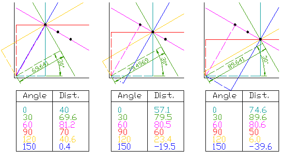
• For each data point, a number of lines are plotted going through it, all at different angles. These are shown here as solid lines.
• For each solid line a line is plotted which is perpendicular to it and which intersects the origin. These are shown as dashed lines.
• The length (i.e. perpendicular distance to the origin) and angle of each dashed line is measured. In the diagram above, the results are shown in tables.
• This is repeated for each data point.
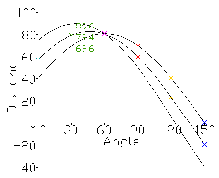
• A graph of the line lengths for each angle, known as a Hough space graph, is then created.

Rate Control at H264

Some applications need constant bit rate (CBR), some need variable bit rate (VBR).
Controlling the output bitrate is typically archived by measuring the rate and/or the encoder buffer fullness level and feeding this back to control the encoder. Many of the encoder parameters can affect output bitrate, like type of slice, motion searching range, mode selection algorithm. The most useful parameter for bitrate control is the quantizer parameter(QP).
One way to control bitrate is simply to try and enforce a constant number of bits per coded frame, by measuring the output bitrate and feeding it back to control QP. This method has problem because it doesn't deal with I,P,B slices separately since they generate significantly  different numbers fo bit, and the image quality may be bad.
A more flexible approach is: the bitrate is used to determine a target number of bits for a Group of Pictures (GOP), typically and I slice followed a number of P/B slices. The bits available for the GOP are then allocated to I,P, and B slices, with the allocation changing depending on the slice type. I slice usually allocate more bits, followed by P slice, and then B slice. Within each slice, a certain number of bits are allocated to each macroblock. The rate control algorithm then attempts to control the encoder to produce the target number of bits. [from book H.264 Adv Video Compression Standard]

CUDA Basic

• Allocate memory:
  

  int *dev_a, *dev_b, *dev_c;
  // allocate the memory on the GPU
  HANDLE_ERROR( cudaMalloc( (void**)&dev_a, N * sizeof(int) ) );
  HANDLE_ERROR( cudaMalloc( (void**)&dev_b, N * sizeof(int) ) );
  HANDLE_ERROR( cudaMalloc( (void**)&dev_c, N * sizeof(int) ) );

  
  
• Copy data to GPU
  
  
  

  // copy the arrays 'a' and 'b' to the GPU
  HANDLE_ERROR( cudaMemcpy( dev_a, a, N * sizeof(int),
                            cudaMemcpyHostToDevice ) );
  HANDLE_ERROR( cudaMemcpy( dev_b, b, N * sizeof(int),
                            cudaMemcpyHostToDevice ) );

  
  
• Run function ‘add( )’ and copy data back from GPU to CPU
  
  
  

  add<<<N,1>>>( dev_a, dev_b, dev_c );
  // copy the array 'c' back from the GPU to the CPU
  HANDLE_ERROR( cudaMemcpy( c, dev_c, N * sizeof(int),
                            cudaMemcpyDeviceToHost ) );
  
  // free the memory allocated on the GPU
      cudaFree( dev_a );
      cudaFree( dev_b );
      cudaFree( dev_c );

  
  
• in ‘add<<<N,1>>>’, N represents the number of parallel blocks in which we would like the device to execute the function. No dimension of launch of blocks may exceed 65,535. The second parameter represents the number of threads per block we want the CUDA runtime to create. The number cannot exceed the value specified by the maxThreadsPerBlock. How to tell which block is currently running?
  
  

  __global__ void add( int *a, int *b, int *c ) {
      int tid = blockIdx.x;    // handle the data at this index
      if (tid < N)
          c[tid] = a[tid] + b[tid]; 
  }

  
  there is no need to define the variable blockIdx, it is one of the built-in variable that the CUDA runtime defines.
• 
  
  Thread: parallel threads within a block will have the ability to do things that parallel blocks cannot do.
  
  

  int tid = threadIdx.x + blockIdx.x * blockDim.x;

  
  
  
  
  
  Because CPU thread management and scheduling must be done in software, it simply cannot scale to the number of threads that a GPU can. Because we can simply create a
  
  thread for each data element we want to process, parallel programming on a GPU can be far simpler than on a CPU.
• 
  CUDA C keyword __shared__ to make this variable
  
  resident in shared memory.  The CUDA C compiler treats variables in shared memory differently than typical variables. It creates a copy of the variable for each block that you launch on the GPU. Every thread in that block shares the memory, but threads cannot see or modify the copy of this variable that is seen within other blocks. This provides an excellent means by which threads within a block can communicate and collaborate on computations. Furthermore, shared memory
  
  buffers reside physically on the GPU as opposed to residing in off-chip DRAM. Because of this, the latency to access shared memory tends to be far lower than typical buffers, making shared memory effective as a per-block, software-managed cache or scratchpad.


• 
  Synchronization: __syncthreads() This call guarantees that every thread in the block has completed instructions
  
  prior to the __syncthreads() before the hardware will execute the next instruction on any thread. When the first thread executes the first instruction after our __syncthreads(),
  every other thread in the block has also finished executing up to the __syncthreads(). In following example, we use multiple threads to calculate the pixel values in a block and displace it. The first image is without using __syncthreads(). This was asked in summer 2009.
  
  
  
  
  
   


• An event in CUDA is a GPU time stamp that is recorded at a user specified point in time.
  
  
  

  cudaEvent_t start, stop; 
  cudaEventCreate(&start); 
  cudaEventCreate(&stop); 
  cudaEventRecord( start, 0 );
  // do some work on the GPU
  cudaEventRecord( stop, 0 ); 
  cudaEventSynchronize( stop );

  
  

HOG

Histogram of Oriented Gradients.

• Use derivative mask [1 0 –1], [1 0 –1]^T in one or both directions of the image. The gradient magnitude will be used.
• A Cell (ex. 6x6 pixels) and a Block (ex. 3x3 cells) are defined as following figure.
• Create oriented histogram bin: the bin can be spread over 0-180 degree if using signed values, and 0-360 degree if using unsigned values. For example, using a 20 degree wide bins, we get 9 bins. Every pixel (use gradient value) inside the cell is used as a weighted vote for the bins.
• Local normalization in block. The normalization factor could be: , where v is the non-normalized vector containing all histograms in a given block, ||v||2 is the 2-norm: , e is a small constant.
• The HOG descriptor is the vector of the components of the normalized cell histograms from all of the block region […,…,…]. The blocks are usually have 1/4 or 1/2 overlaps. 

HOG is widely used descriptor due to the speed of computations, inherent robustness to slight object variation/deformations, and the ability to capture a coarse spatial layout of features.

Update: 4/17/2012
Some implementation details:
Suppose the image size is 320x240, cell size is 8x8, so we have 40x30 blocks.  Suppose 18 orientations are used, we define two vectors for x,y directions:

double uu[9] = {1.0000, 

        0.9397, 

        0.7660, 

        0.500, 

        0.1736, 

        -0.1736, 

        -0.5000, 

        -0.7660, 

        -0.9397};

double vv[9] = {0.0000, 

        0.3420, 

        0.6428, 

        0.8660, 

        0.9848, 

        0.9848, 

        0.8660, 

        0.6428, 

        0.3420};

To check which orientation the current pixel locates at:

loop dx, dy within image size

double best_dot = 0;

int best_o = 0;

for (int o = 0; o < 9; o++) {

    double dot = uu[o]*dx + vv[o]*dy;

    if (dot > best_dot) {

      best_dot = dot;

      best_o = o;

    } else if (-dot > best_dot) {

      best_dot = -dot;

      best_o = o+9;

    }

}

Create the histograms for 18 orientations.  The pixel values in each orientation are added up.

Computer energy in each cell by summing over orientations

Output features. The features could be:

contrast-sensitive features (size 18): it is the pixel energy in each orientation

contrast-insensitive features (size 9): the energy in each orientation (no sign)

texture features (size 4): check the neighbor 4 pixel energy 

So the output features size is 40x30x31. (31=18+9+4)

Scale Space

Scale space is the space of measurements that you can get after blurring image by successively larger and larger Gaussian kernels.

Smooth away noises by blurring image is to make measurements at large scales (or say we use a larger apertures). So it gets above the scale of the noise, and only make measurements at scales more natural for objects in the image.

Image pyramid.

Review of Edge Detectors

1st derivative methods:

• Roberts Kernels
• Prewitt
• Sobel

2nd derivative methods:

• Laplacian Operators
• Laplacian of Gaussian
• Difference of Guassians

Difference of Gaussians (DoG)

Subtracting a wide Gaussian from a narrow Gaussian.
In edge enhance applications, a high pass filter is used. The high pass filter can also enhance the noise which also has high frequency. Difference of Gaussians remove high frequency content of noise. So it is a good method for edge sharpening, image enhancement.
The drawback is that it reduces the overall image contrast.
The practical kernel size for two gaussian (ratio) is 4:1, or 5:1.
DoG is very similar with Laplacian of Gaussian. It will get similar result when the ration is 1.6.

[update: 2/19/2013] the DoG is actually a band-pass filter, which removes high frequency components representing noise, and also some low frequency components representing the homogeneous areas in the image

3 image features for content based image retrieval

All are from MPEG-7.
Scalable Color Descriptor: a color histogram in HSV color space. For example, Hue is divided into 8 fuzzy areas: (0) Red to Orange, (1) Orange, (2) Yellow, (3) Green, (4) Cyan, (5) Blue, (6) Magenta and (7) Blue to Red. S is divided into 2 fuzzy regions, The first area, in combination with the position of the pixel in channel V, is used to define if the color is clear enough to be ranked in one of the categories which are described in H histogram, or if it is a shade of white or gray color.
Color Layout:
Edge Histogram Descriptor: the filters for edges from different angles:

• vertical: [1 –1; 1 –1]
• horizontal: [1 1; –1 –1]
• 45 diagonal: [sqrt(2) 0; 0 -sqrt(2)]
• 135 diagonal: [0 sqrt(2); -sqrt(2) 0]
• non-directional: [2 –2; –2 2]

the respective edge magnitudes are ‘m_xx’, each image block is derived to 4 sub blocks, the average gray level of each sub block is a_x(i,j), where x is 1,2,3,4, then m_xx = | sum_0^3 a_x(i,j) * f_x(k) |, where xx is vertical, horizontal, etc., and its max value is ‘max’. We get the edge histogram with:

if (max < TEdge) EdgeHist[0]++; // no edge
else                            // different direction
if (m_nd > T0) EdgeHist[1]++;
if (m_h  > T1) EdgeHist[2]++;
if (m_v  > T1) EdgeHist[3]++;
if (m_45 > T2) EdgeHist[4]++;
if (m_135> T2) EdgeHist[5]++;

wildcard query: permuterm index and k-gram index

Let “$” mark the end of a term such that “hello” –> “hello$”. The permuterm entry for term “hello” are:

hello$, ello$h, llo$he, lo$hel, o$hell, $hello

In a wildcard query “m*n”, rotate the query so that the “*”appears at the end of the string. So “m*n” changes to “n$m*”. The look up this string in the permuterm index. Seeking “n$m*” leads the rotations of the terms “man” and “moron”.

When query X, look up on X$, query X*, look up on $X*

*X –> X$*, *X* – > X*, X*Y –> Y$X*

That means: rotate wildcard query to the right and use B-tree to lookup.

permuterm index need a lot of space.

--

In a k-gram index, the dictionary contains all k-grams that occur in any term in the vocabulary. For example, the 3-gram “etr”would point to terms sucha as: retrieval, petrify, metric, beetroot.

Use “$”as a special word boundary symbol. The 2-grams in text “the month” are: $t, th, he e$, $m, mo, on, nt, th, h$”

In wildcard query “mon*”, run as: $m AND mo AND on

Postings list intersection with skip pointers

The list lengths are m and n. If we go through the two posting lists simultaneously, it takes O(m+n) operations. With skip pointers:

In following figure, when we reach “8” and move it to the result list, the next pointers are “16” and “41” in upper/lower list. Rather than simple advancing the upper pointer, we found the skip list pointer “28” is also less than “41”. Hence we can follow the skip list pointer and advance the upper pointer to “28”, thus avoid to “19,23”.

Now how many steps to skip? suggestion is sqrt(p), where p is the posting list length. The algorithm is:

Dictionary data structure in IR

If using an array, it looks like:
term ---- document freq. ---- pointer to postings list
a       |       34594          | pointer
..
as     |    32423             |
..
zzz   | ....

The three parts are 'char[20], int, postings *', the sizes are 20 bytes, 4 bytes, and 4 bytes (or 8)

In IR systems, Hash table or Tree is used.
Hash table: each vocabulary term is hashed to an integer, the lookup time is O(1). The problems are: not easy to find minor variants, no prefix search (tolerant retrieval), and if vocabulary growing, need to rehash everything.

Trees: B-trees is more usual than binary tree. This solves the prefix problem, but the search time is O(logM).

Information Retrieval (IR)

Information retrieval is finding material (specific documents) of an unstructured nature (text) that satisfied an information need from within large collections.
IR vs. Database: structured vs. unstructured data. Structured data tends to refer to information in 'tables', unstructured data typically refers to free text, allows keyword queries including operators, sophisticated concept queries.

Indexer steps: dictionary, postings, and document frequency information (freq used for query optimization).
Query steps: for example "aaa AND bbb".

1. locate aaa in the dictionary, retrieve its postings (postings sorted by docID)
2. locate bbb in the dictionary, retrieve its postings
3. merge the two postings: walk through the two postings simultaneously, if the list lengths for aaa and bbb are x and y, the merge takes O(x+y) operations.

while p1 != NULL && p2 != NULL
do  if  docID(p1) == docID(p2)
      then add docID(p1) to answer
else if docID(p1) < docID(p2)
then p1 = next(p1); p2 = next(p2);

In general query (aaa AND bbb AND ccc), we should start with the smallest document frequency, then keep cutting further. 

Basic indexing pipeline: Documents to be indexed -> (Tokenizer) -> Token stream -> (Linguistic modules) -> Modified tokens -> (Indexer) -> inverted index

Tokenization
A token is an instance of a sequence of charcters, each token is a candidate for an index entry. (input:friends, romans and countrymen", output tokens: friends, romans, countrymen

Normalization to terms
A term is a normalized word type, which is an entry in IR system dictionary. You have to normalize indexed text and query terms into the same form.

Stemming suggest crude affix chopping ("compressed, compression ..." -> compress). Porter's algorithm.

Biwordk indexes for phrases

Use CLucene

1. create a new project with 'Win32 Console Application'
2. add 'new project...' with CLucene
3. in property of Solution, change 'Project Dependencies', your project depends on CLucene
4. edit stdafx.h, stdafx.c with the same content of Demo
5. in property pages of your project:

• C/C++ General: ../../src;../../src/yourProj
• Preprocessor (maybe)
• Code Generation: Runtime library - /MTd
• Precompiled Headers: Not using (maybe)
• Liner General: Enable Incremental Linking - Yes (/Incremental) (maybe)
• input: Additional Dependencies - ../../build/lib/clucene-coreUDMT.lib

If you got the error "defaultlib 'LIBCMTD' conflicts with use of other libs; use /NODEFAULTLIB:library", you may try change the Runtime library with '?MTd'
If you got the link error "IndexFiles.obj : error LNK2019: unresolved external symbol "public: char * __thiscall lucene:: ....", something was wrong with the very first step. Try to New a  'Win32 Console Application'.

Intra prediction and Inter Prediction Performance

If you get better compression performance (P-frame), you need more computation.
If you get better computation performance (I-frame), you get worse compression. (I dont' know why I added P-frame and I-frame there. These compression performance/computation thing works for both of them. It is a trade off [8/1/2012])

In general, inter prediction gets the better compression performance.
Intra prediction is not the best prediction. But in some cases, such as the very first frame, we have to use intra prediction.
Intra prediction can get better performance too, e.g., in very complicated video scene, such as smoke, explosion, it is very difficult to use inter prediction. Another example, when you random access the point of a video, you want to use intra to start from there.
I-frame: a random access unit.
[update 8/1/2012]: If only using p-frames, the reconstruction errors will accumulate. An I-frame is required for every N frames, N depends on the application, N=15 or 30 in my case.

Thermal Camera

Three categories in infrared light:

• near-infrared (near-IR)
• mid-infrared (mid-IR)
• thermal-infrared (thermal-IR)

The key difference between thermal-IR and the other two is that thermal IR is emitted by an object instead of reflected it. 

The ability to emit energy ranges 0-1, depending on the properties of materials. The blacker material has the value close to 1. The reflective material has a lower value. For instance, polished silver is 0.02, iron has 0.14 if polished, and 0.61 if rested. Regular glass, which effectively blocks thermal radiation, has 0.92.

The thermal radiation also depends on its temperature, the hotter thing emits more thermal radiation. 

Run Length Encoding (RLE)

The same color pixels in one row (or column, zigzag) are coded with a counter and pixel value. For example, aaabccccccddeee is coded to 3a1b6c2d3e

That is lossless data compression. It works well if the pixel values are the same in large regions. If every two pixel values are different, the algorithm will double the data, instead of compression.

JPEG

Basic BMP -> JPG process:

BMP -> YUV 420
YUV420 sampling. Using one 16x16 mcu, and six 8x8 DU: Y0,Y1,Y2,Y3,U,V
DCT to every DU
Quantize DU using table, zigzag scan
Huffman coding and get bits
Write bits to file

Y/U/V components of an image, which use fixed sampling factor 2x2 for Y (luminance), and 1x1 for U/V (chrominance). Using this sampling scheme, each pixel will only require 12 bit to record the color (2 pixels = (4Y + 1U + 1V)*4 = 24 bit, 1 pixel = 12 bit).

For each component, a DU (data unit) in JPEG represents a 8x8 byte matrix, by using huffman coding the zigzaged 64 FDCT coefficients;

By using the YUV12 sampling scheme, a MCU (minium coded unit) in JPEG represents a 16x16 (pixel) image block, by using 6 DUs in this sequence: YDU, YDU, YDU, YDU, UDU, VDU.

default quantization tables for luminance and chrominance
provided by "ISO/IEC 10918, 1993(e)" Annex K:

luminance quantization table:

16 11 10 16 24 40 51 61
12 12 14 19 26 58 60 55
14 13 16 24 40 57 69 56
14 17 22 29 51 87 80 62
18 22 37 56 68 109 103 77
24 35 55 64 81 104 113 92
49 64 78 87 103 121 120 101
72 92 95 98 112 100 103 99

chrominance quantization table:

17 18 24 47 99 99 99 99
18 21 26 66 99 99 99 99
24 26 56 99 99 99 99 99
47 66 99 99 99 99 99 99
99 99 99 99 99 99 99 99
99 99 99 99 99 99 99 99
99 99 99 99 99 99 99 99
99 99 99 99 99 99 99 99

In quantise: where vector is raw data, qt is the table.
for(i = 0; i <>

Sub-pixel motion vectors in H.264

The offset between the two areas has 1/4 pixel resolution for the luma component, 1/8 pixel resolution for choma component. In following figure, A,B,C… are regular pixels and b,h,m… are half pixle. The half pixle can be calculated with 6 weighted filter, the weight is (1/32, –5/32, 5/8, 5/8, –5/32, 1/32). To get ‘b’:
b = round ((E – 5F + 20G + 20H –5I + J)/32).
We can get ‘h’ from A,C,G,M,R and T. Then ‘j’ can be calculated from cc, dd, h, m, ee, and ff.

After 1/2 subpixel is calculated, we can get 1/4 subpixle with interpolation. In following figure, a,c,i,k,d,f,n,q are from interpolation. For instance:
a = round((G + b) / 2)

The other 1/4 sub-pixel (p, r…) can be calculated from  diagonal pixels. For instance, e is from b and h.

1/8 sub-pixel is required in choma motion vector component. It also uses linear interpolation.
a=round(( (8-dx)*(8-dy)*A + (8-dy)*B + (8-dx)*dy*C + dx*dy*D) / 64)